Experimental Procedure
Recording Solutions
Slice dissection and recording takes place in artificial cerebrospinal fluid (ACSF) solutions (See Table 1). These solutions consist of salts, pH buffers, energy sources, and divalent ions. Experimenters often adjust their solutions for different purposes. The replacement of sodium with NMDG or sucrose during slice preparation can improve the survival of cells in the slice (Tanaka et al., 2008), both in the brainstem and cortex. Replacing sodium ions prevents cells from spiking, reducing excitotoxic damage, and reduces the activity of Na+/K+ pumps, reducing metabolic demand. Sodium pyruvate and myoinositol provide alternate entry points into cellular metabolism, and their addition seems to improve cell survival. Ascorbic acid acts as a free radical scavenger and may help cell survival. Ascorbic acid may be required in experiments that use drugs sensitive to free radicals.
While the divalent ion concentrations listed in Table 1 are common in brain slice experiments, it is important to recognize that these are significantly higher than those occurring in vivo. Recent experiments in the medial nucleus of the trapezoid body at the calyx of Held have revealed how the use of these high divalent concentrations can lead to conclusions from in vitro studies that may not apply in vivo (Lorteije et al., 2009). The use of high divalents dates from the early days of slice recording, where it was found that elevated calcium seemed to help with forming seals between cell membranes and pipette glass. The elevated calcium concentration also increases release probability at synapses, which makes synaptic responses larger and more reliable. However, solutions with a more “physiological” calcium and magnesium, such as 0.8 mM CaCl2 and 1.3 mM MgSO4, can ease the interpretation with respect to in vivo conditions. Alternatively, it is important in some experiments to provide both high release probability and low polysynaptic transmission, which can be achieved by using even higher calcium and magnesium (4 mM). Such concentrations are often used in photostimulation experiments where spatial maps of connectivity are the primary goal and time constraints prevent repeating maps many times to measure connections with low release probability.
When making ACSF, the components are added in the order given in Table 1, and are weighed out on a balance (with 0.1 mg resolution) as accurately as possible. Between uses, salts are stored in a dessicator to minimize water absorption. The divalent ions are added last, just before use, to prevent precipitation. This solution is either warmed to 34 °C in temperature controlled water baths, or chilled in a freezer for 30-45 minutes before use. The solution should be oxygenated and pH equilibrated by gassing with 95% O2 - 5% CO2. The pH should be between 7.35 and 7.40. Inadequate gassing can lead to a more basic pH, and can be a cause of poor slices. We do not recommend making “stocks” of the incubation and recording solutions for three reasons. First, without equilibration with 95% O2 - 5% CO2, the solutions will become basic over time, which causes the divalent ions to precipitate out of solution. Second, with the sugars in the solution, it does not take long to get bacterial growth, and bacterial endotoxins are not conducive to good slice health. Third, if a stock is incorrectly prepared, several days’ (or even months’) worth of experiments may be disrupted. With practice, it only takes about 15 minutes to prepare 1-2 L of solution, and this is readily done on the morning of each experiment.
Electrode Solutions
Pipettes are filled with an electrolytic solution whose primary function is to conduct current between the electrode and the interior of the cell (or exterior membrane surface). Because patch electrodes also facilitate the exchange of soluble molecules, pipette solutions used in intracellular recordings are designed to mimic the contents of the cytosol (or CSF, in the case of cell-attached patch) to preserve the natural function of the cell. Pipette solutions vary according to the goals of the experiment, and this is an aspect of the experimental design that requires some consideration. Standard recipes for potassium gluconate and cesium solutions are given in Table 2. Potassium gluconate is generally used for current clamp experiments, when normal cell activity is desirable. For voltage clamp, cesium based solutions are often used because Cs+ ions block K+ channels, which increases the length constant of the cell (see Section 4.7.6). QX-314, a Na+ channel blocker, is often added to cesium-based solutions to block action potentials.
Electrode solutions are usually used in small quantities, and so are prepared in batches, and stored in single use aliquots of 100 or 200 μl at -80 °C. The usable lifetime of an electrode solution is ~3 months, although this may vary with the content. When retrieving the solutions from the freezer, it is important to vortex each solution, since during freezing components may come out of solution or a gradient in osmolarity may appear. The solution should then be centrifuged briefly to pull down any debris. Alternatively, or in addition, the solutions can be passed through a 0.22 μm filter. The solution is then stored capped in an ice bath during use, and is discarded at the end of the day. The pipettes are filled as needed immediately prior to use. We have found that filling pipettes in batches that sit all day prior to use usually leads to low success rates.
The filling solutions used for patch work are often slightly hypoosmotic with respect to the bath. There are two reasons for this choice. First, as a seal is made onto a cell, the higher osmolarity in the the cell relative to the pipette helps push the cell membrane closer against the pipette tip, aiding in forming a seal with less hydrostatic pressure. Second, a portion of the cell’s osmolarity is made up of elements with low diffusibility, so using a lower osmolarity in the pipette itself is less disruptive and less likely to lead to cell swelling over time.
Many electrode solutions used in patch clamp recording have unusual combinations of ions, particularly anions, that introduce electrochemical potentials both at the electrode tip and between the solution and the wire that connects to the headstage. These potentials interfere with the accurate measurement of the cell membrane potential. While the potential between the wire and the electrode solution can be eliminated by adjusting the offset controls of the amplifier easily enough, the tip potential can be problematic and it is necessary to know its value in order to know the proper membrane potential of a cell in either current or voltage clamp. The tip potential is different when the cell is in the bath, and when it has access to the cell, since the electrochemical potential in the two conditions is different. Typically the tip potential has to be measured. One way to do this is to place a filled electrode into a bath containing the electrode solution, and using an amplifier in current clamp, measure the potential. Next, while keeping a very slight amount of positive pressure on the electrode to minimize mixing with the bath solution, exchange the bath for a normal extracellular solution, and measure the potential again. The difference is the tip potential that would exist when the electrode is in the bath, but which (mostly) dissipates when the electrode is in the cell. Typically, for a 140 mM K-gluconate based electrode solution with low (4-8 mM) KCl, this potential will be about -12 mV. This means that, if the electrode potential is set to zero outside the cell, and measured at -50 mV (or clamped to -50 mV) when the electrode accesses the cell, the actual resting (or holding) potential is -62 mV.
Patch Electrodes
Standard patch clamp electrodes are made from borosilicate glass pipettes which are heated and stretched to form a pipette with a blunt tip ~1-2 μm in diameter (figure 4). Since patch electrodes can only be used once and have a very limited lifespan, they are most often made on-site using programmable pipette pullers. These pullers work by heating and melting the center of a glass pipette and pulling the two halves away from each other to form two identical tapered electrodes. The exact shape of the electrode is determined by the timing and power of heating as well as pulling force. Two competing factors must be considered and balanced when pulling pipettes. First, the shape of the pipette determines its electrical resistance and capacitance, both of which should be minimized to improve recording fidelity. Typical pipettes have a resistance of 2-10 MOhm and capacitance of only a few pF. Second, pipette tips that are too large (>2.5 um) or too small (<1 um) may be difficult to patch with or unable to maintain long-term access to the cell.
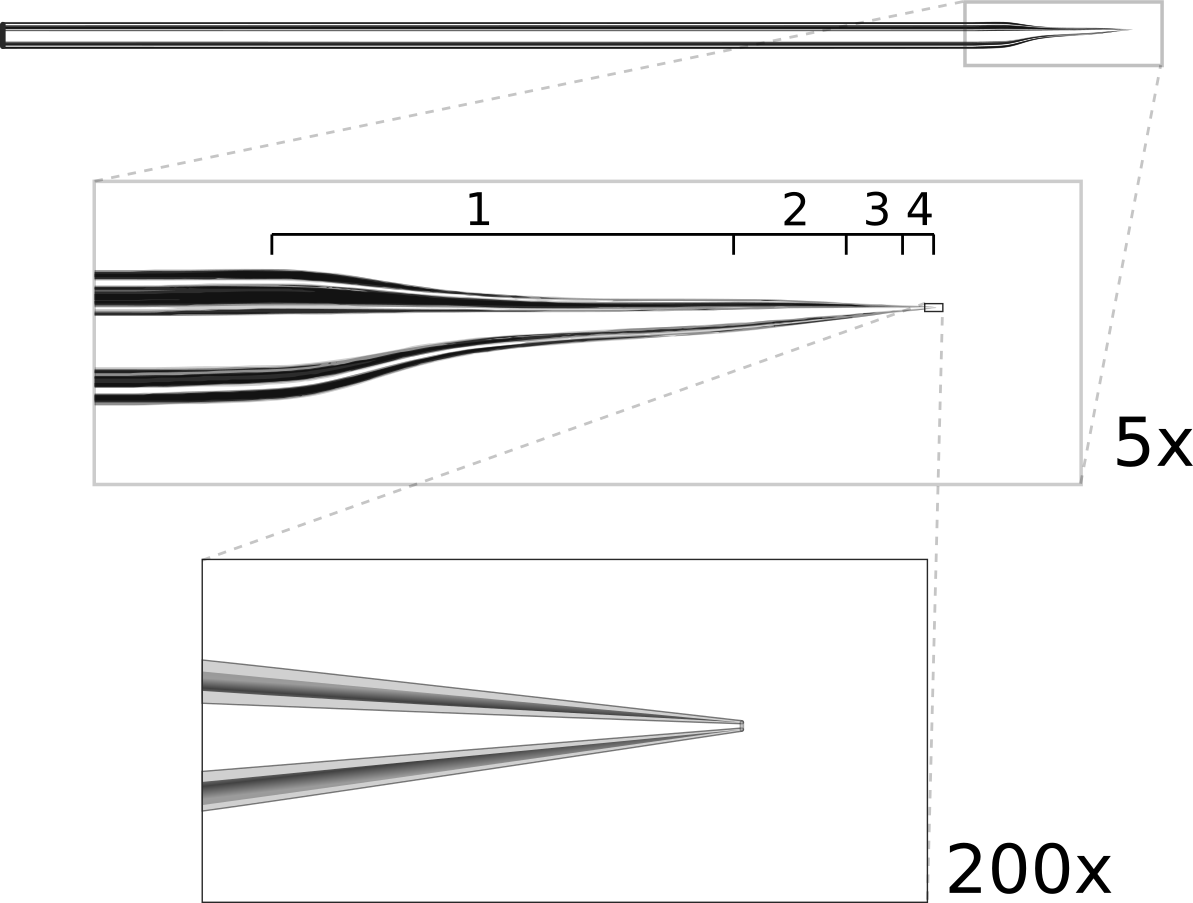
Ideal patch pipette shape. The pipette is pulled in multiple stages. The first stage is a long, narrow pull which thins the tip to help it fit under the objective. The following stages produce a rapid taper (about 15°) to reduce resistance and end with a 1.5μm tip.
The resistance of a patch pipette is inversely proportional to both the angle and diameter of the tip (approximated as a conical conductor). Thus to reduce resistance, both values should be maximized; however, tip diameters greater than ~2 μm may be difficult to patch with. With the tip pulled to ~15°, it should be possible to produce pipettes with low resistances around 2-5 MΩ. Such low resistance is crucial for voltage-clamp experiments measuring currents greater than a few hundred pA, such as evoked synaptic currents or currents through ion channels. For current clamp recordings, higher resistances up to 20 MΩ may be acceptable as long as the access resistance to the cell is stable for the duration of the recording.
Another factor to consider is that the pipette must fit comfortably between the objective and the recording chamber (see figure 3). For objectives with a short working-distance, it may be necessary to reshape the pipette tip. We shape tips by pulling in multiple stages: the first stage produces a long, narrow pull and subsequent stages taper the tip more quickly (figure 4). The long first stage provides more room under the objective but does not significantly increase the resistance because the last 100 μm of the tip accounts for roughly 95% of the total resistance.
The choice of glass can be important in some experiments, and so familiarity with the different compositions made by different manufacturers can be helpful. Typical pipette glass is borosilicate-based, and will have an outside diameter of 1.0-2.0 mm, and an inside diameter of 0.5-1.6 mm. The thickness of the glass wall is generally maintained in proportion to the diameter of the tip as the glass is pulled, and for patch-clamp recording, thicker walled glass is generally preferable to reduce pipette capacitance. Patch pipette glass often includes a small interior filament that acts as a wick to draw electrode solution into the tip. Some pipettes are produced with the raw ends fire-polished. This is necessary to prevent the otherwise sharp glass from scratching the thin AgCl layer on the silver wire. Pipettes can be easily polished by holding the back end over a small flame for a few seconds, until the glass glows orange.
Producing clean, correctly-shaped pipettes often requires much trial and error. Once pipettes are pulled, they may be individually inspected under 10X and 40X objectives. This screening process is used both to guide adjustments to the puller to obtain the desired diameters and tip shapes, and to discard pipettes that are broken, fouled or which fall outside the desired tip diameter. It is of the utmost importance that the tips of patch electrodes be clean. Thus, pipette blanks should only be handled by the ends to avoid placing skin oils in the region that will be heated. Pulled pipettes are only used on the day they are made, because of increased chances of tip fouling and potential hydration of the fine tip glass that could affect the dielectric properties of the glass and introduce recording noise.
An optional final step in preparing pipettes is to coat the tip to reduce capacitance to the bath and improve the dielectric properties. The effect of the coating is to reduce recording noise, and to improve the ability to fully and properly compensate the electrode capacitance for voltage-clamp recordings. When performing voltage-clamp studies, we consider the application of a coating essential. In experiments in which only current-clamp recordings are done, this step can be skipped, although the reduction of capacitance reduces the amount of compensation needed, which in turn reduces the overall noise level of the recording. There are two approaches that are commonly used. The first is to use a conformal coating, such as Sylgard (Dow Corning 184). This is a two-part mixture that can be painted to within 50 μm of the tip using a fine needle while viewing the tapered region of the pipette with a dissection microscope. The mixture cures in several seconds by applying heat (we use a paint stripper on its low setting). The Sylgard can also be stored uncured in the freezer (-20 °C) for about 2 weeks, and we find that preparing the mixture about 24 hours prior to first use is also helpful. A second approach is to wrap the tip of the pipette with a 2-3 mm wide strip of Parafilm, which can be melted with gentle heat, or to dip the tip of the pipette in molten parafilm, while keeping positive pressure on the pipette to maintain a clear tip.
Filling the pipette with electrode solution is also an important step and one where problems can occur. While there are various commercial filling needles, these tend to be expensive and hard to keep clean, often leading to clogged electrodes. A different approach is to use 100 μl pipette (those made with a harder plastic seem to work best), tips pulled over a flame to create a very fine tube (figure 5AB). With care and practice, these make filling tips that are only a few hundred μm in diameter. The fillers can be inserted into a 1 ml syringe and backfilled from the electrode solution stock (figure 5C) or capped over a pre-filled syringe and filter (figure 5D). The major advantages of these fillers are that they are disposable if they become dirty, are economical, and are easily remade. For making fillers and fire polishing pipettes, we have created a small burner from an 18-gauge blunt needle that provides a flame size similar to a match.
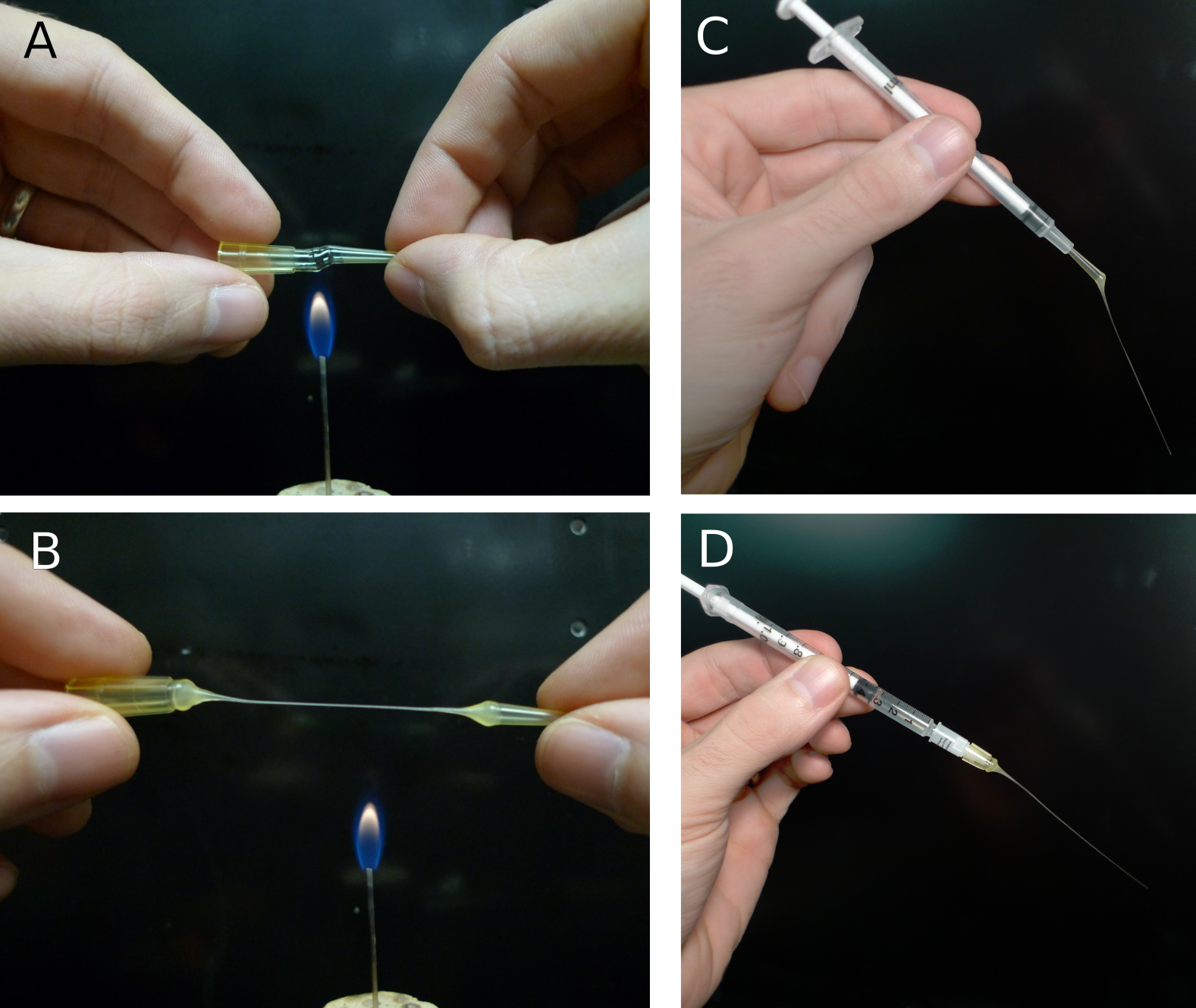
Figure 5. Making patch pipette fillers from disposable pipette tips. A) Heating a 100 μm disposable pipette tip over a small flame. The tip should be rotated to produce even heating and care should be taken to avoid burning the plastic. B) As soon as the tip has melted through, remove it from the heat and pull into a thin tube (this takes some practice). Cut the tube with a sharp blade to avoid crushing it. C) Filler made from tip of pipette inserted into 1 ml syringe. D) Filler made from base of pipette attached to 1 ml syringe and a low-volume, 0.2 μm-pore syringe filter.
Dissection and Slicing
The preparation of brain slices containing healthy cells is critical to the success of patch recording. The goal is to extract a section of the brain such that the cells of interest are close to the surface of the slice and any other required network connections are intact elsewhere in the slice. Furthermore, we need to make sure that the cells/tissue are still sufficiently alive and undamaged and that they can be visualized well enough to facilitate patching. Producing viable brain slices can be very difficult and proven methods often vary widely between brain regions. The main factors affecting slice viability are: 1) Prevention of ischemic damage by dissecting and slicing quickly, often in well-oxygenated, ice-cold ACSF (the ACSF may actually be partially frozen). 2) Prevention of excitotoxic damage through use of specialized ACSF solutions. 3) Prevention of mechanical damage by avoiding compression/stretching of brain tissue and by using well-tuned slicers with appropriate blades.
Blades: The choice of cutting blade can be critical to successful slice preparation, especially in older tissue. The most commonly used blades are commercially available double-edged stainless-steel razor blades. These vary in quality however, and different types should be tried to determine which ones work best for a specific brain region. “Platinum plus” blades have worked well in the brainstem and cortex, while other types of blades have been found to yield very poor cutting. Reusable blades made of sapphire or ceramic are also excellent choices, especially if they can be resharpened. Blades should be cleaned prior to use, and stainless-steel blades should only be used for one cutting session. Cleaning is necessary to remove oils and other protective chemicals used to retard oxidation and corrosion of the blades. We clean by first briefly washing the blade in acetone with a cotton swab, followed by a 70% ethanol rinse, and finally a distilled water rinse. The blade is then dried, and placed in the chuck of the slicer.
We discuss preparation of slices from two different brain regions below, to illustrate two different approaches to creating viable brain slices. The first method, for neocortex, follows a conventional approach, while the second method, which we use for cochlear nucleus, demonstrates how variations on the procedure may be best applied for different brain regions. Prior to removing the brain, all solutions need to be at an appropriate temperature and properly oxygenated, surgical tools should be located and clean, and the cutting blade should be in place. The goal is to make the time between decapitation and the incubation of the slices in the holding chamber as short as possible. At the same time, it is critical to be careful with the tissue, and to handle it gently. In each approach, the animals are first deeply anesthetized, according to an approved protocol, and decapitated.
Cortex: The skull is exposed, cut down the midline with fine-tipped scissors, and peeled back with rongeurs (in adult animals where the skull is thick) or with fine-tipped scissors (in younger animals when the skull is thin). Care should be taken not to touch the brain itself when removing the skull. The brain is removed after carefully cutting major cranial nerves that may enter or leave near the tissue of interest. The brain is then “rolled” out using a small spatula, into an ice-cold dissection solution (see below for composition). The tissue is trimmed, using fine scissors and scalpel blades. The key elements in trimming are to obtain a flat surface that is parallel to the desired plane of section that can be used to glue the brain block to the stage, and to remove any excess tissue that does not contribute to stabilizing the brain block during cutting. It is helpful to have a specific sequence in which the trimming is performed, as with practice this can greatly speed the preparation.
The next step is to place the tissue block on the chuck that will go into the slicer. We usually prepare the mounting position by laying down a small platform made of 4% agar (made in 150 mM NaCl) to support the tissue, and place an agar wall behind the platform. In some cases, these agar supports are cut with an angled surface to help orient the brain when it is glued down. A drop of cyanoacrylate glue is placed on the platform just in front of the wall. The tissue is then picked up by sliding it onto a small piece of ashless #50 filter paper (this paper is “hard” and can hold small blocks of tissue even when wet), such that the part of the tissue that will be against the wall is against the tissue paper. The chuck is placed at an angle such that the wall can support the tissue by gravity. The tissue block is then transferred onto the cutting chuck by sliding it against the wall until it comes in contact with the glue, at which point the filter paper is slid out from under the tissue. It is important in this step that the glue not come in contact with the filter paper. We next mount 4% agar support blocks (usually ~2x2x6 mm posts) that are glued to the stage and gently abut the tissue, to minimize movement of the tissue during cutting. Cutting takes place in a cold solution in a previously frozen cutting chamber surrounded by an ice slurry.
Brainstem (cochlear nucleus): The squamous portion of the occipital bone over the cerebellum is removed with rongeurs (fine scissors are sufficient in mice), exposing the cerebellum and brainstem. The brainstem is briefly washed with warmed oxygenated ACSF. The temporal bone is carefully retracted laterally, the floccular and parafloccular lobes of the cerebellum are gently lifted, and the exposed eighth nerve (both the auditory and vestibular branches) is then sectioned with the tip of a #11 scalpel blade. Care is taken to minimize stretch of the nerve while cutting. The brainstem is transected rostral to the inferior colliculus with a spatula, and again caudal to the obex, removed from the skull, and rinsed again in ACSF. A small tissue block containing the cochlear nucleus of the left side is then isolated from the brainstem. The brainstem is bisected at the midline longitudinally with a scalpel, and trimmed rostral and caudal to the cochlear nuclei with scissors. The choroid plexus lying above the cochlear nucleus is gently teased away with #5 forceps. Most of the cerebellum is cut away at the cerebellar peduncles with scissors. The rostral and caudal ends of the block are trimmed at an angle approximately parallel to the long axis of the cochlear nucleus. A final cut is made parallel to the desired cutting plane; this may be along the midline or across the ventral surface. This block is transferred using a strip of hardened #50 ashless filter paper, blotted to remove excess fluid, and mounted on the chuck of the tissue slicer with cyanoacrylate glue. The tissue is supported with agar blocks from behind and on the sides. The chuck and tissue are immersed in a warmed carbonated cutting solution in the bath.
For either tissue region, slices are cut by carefully advancing the blade into the tissue under visual control. Often, a few 500 μm thick slices are quickly taken until the desired region is reached, and then the cutting thickness is adjusted to 250-350 μm, and a series of slices collected. As each slice is taken, it is checked under a dissecting microscope to be sure that it is from the appropriate region and is not damaged, and then is transferred to the incubation chamber using the blunt end of a Pasteur pipette whose tip has been broken off and fire polished so a pipette bulb can be attached. We prefer this method over using small paint brushes, as there is less mechanical stress to the tissue slice during the transfer.
Slice Incubation
Slices are commonly allowed to incubate for 30-60 minutes at 32-34 °C after slicing to allow them time to recover and re-equilibrate to the ACSF environment. After this the slices are usually incubated at room temperature. The slices are held in an incubation chamber that may be in a water bath, or on the bench for room temperature incubation. We primarily use a simple chamber that consists of a 100 ml glass beaker. A sintered-glass gas dispersion tube is inserted into the chamber and about 60 ml of ACSF is added, and well gassed with 95% O2-5% CO2. The slices rest on a permeable nylon mesh that forms the bottom of multi-well tray. This tray is hung in the chamber so that the ACSF covers the mesh, but is 1-2 mm from the top of the tray walls. The top of the chamber itself is loosely covered with parafilm to minimize evaporation over time. Other incubation chambers have been used as well. The key requirements are that bathing solution is exchanged around the slices by a stirring action (usually provided by the gas dispersion system), that the solution is well gassed, that evaporation is controlled, and that the chamber and gas dispersion system does not leach chemicals into the incubation solution.
Recording chamber / perfusion / harps
After incubation, slices are held in a small volume (~0.3 ml) recording chamber mounted on the stage of an upright microscope. The slice rests either on a coverglass or on a small section of netting, and is held in place by another net stretched across a stainless steel harp. Warm, oxygenated ACSF is perfused over the slice at 2-8 ml/min by siphoning from a flask. The incoming perfusate is warmed to 38 °C just prior to entering the chamber with a feedback controlled heater, resulting in a solution temperature at the slice of 33±1 °C. While some experimental procedures, such as analysis of network organization using photostimulation, can be done at room temperature, it is nearly always preferable to record at elevated temperatures to more closely approximate the normal kinetics of ion channels, the release properties of synapses, and the engagement of intracellular signaling cascades.
The fluid level in the recording chamber is regulated by positioning an aspirator above the surface of the water. While a properly configured aspirator should maintain the bath at a constant level, it is nevertheless important to monitor the chamber to avoid overflows which may damage equipment or underflows which may damage the slice.
To prevent electrical noise, it is very important that the fluid in the recording chamber be electrically isolated from everything except the patch and ground electrodes. If the chamber overflows, it is possible this will create a new electrical path to ground or other parts of the setup, introducing a new potential noise source.
Patching
Finding viable cells
You are finally ready to patch a cell. The first task, then, is to find a cell that appears to be healthy and is in the correct location of the slice. The appearance of healthy cells will vary somewhat between brain regions, but typically these will appear to have a smooth, translucent interior and a smooth cell membrane (figure 6, white arrows). Unhealthy cells often appear either shriveled or bloated, have a rough or abnormally transparent interior, or have a visible nucleus and nucleolus (figure 6, black arrows). However, these features are not always diagnostic of cell health and it is possible to bias the cell selection by avoiding healthy cells with an abnormal appearance. Ultimately, trial and error may be the best way to determine which cells can be patched successfully, and which appearances are associated with healthy cells. In a few cases, the situation may call for alternative methods such as shadow patching (using fluorescent electrode solution and looking for dark regions indicating a healthy cell that is impermeable to fluorophore) or blind patching (using electrical signals rather than visualization to determine when the pipette has contacted a cell) instead of direct visualization.
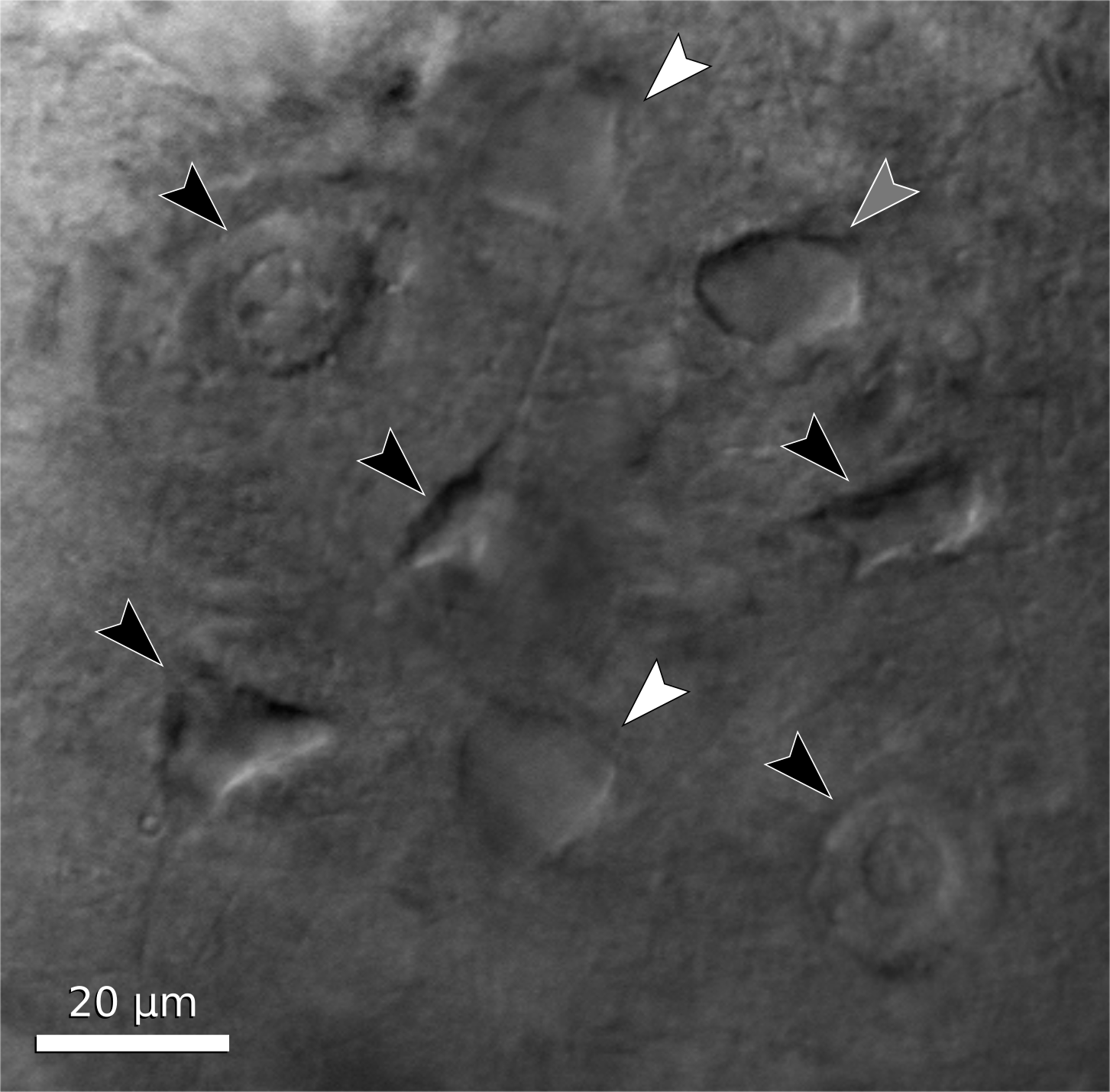
Figure 6. Neuron examples in a cortical brain slice under gradient illumination. Black arrows indicate unhealthy or dead cells, white arrows indicate healthy cells, and a grey arrow indicates a borderline cell. (This figure is a composite of multiple images from different regions of a slice.)
It is preferable to avoid cells very close to the slice surface, as they are likely to have been severely damaged during slicing. Generally, one should attempt to patch cells as deep as possible given the limitation of visibility in the slice. For relatively transparent tissue such as neocortex from young animals, it may be possible to visualize cells up to 50-100 μm deep. For older or heavily myelinated tissue, visibility may be limited to 20 μm or less. In this situation, having properly adjusted illumination and a good camera is crucial. It may also be necessary to use software that allows large contrast adjustments or background subtraction.
Once a candidate cell has been selected, center the cell within the camera’s visible range and switch back to a low-power objective in preparation for positioning the patch pipette.
Filling patch pipettes
For each cell you wish to record, a new patch pipette must be prepared and filled with electrode solution. It is recommended to make all patch pipettes at the beginning of the day (about 6-12 should suffice, depending on the experiment) but do not fill the pipettes with electrode solution until immediately before each is to be used. The day’s aliquot of electrode solution should be thawed, vortexed, centrifuged, and kept chilled on ice. Note that vortexing is critical because just-thawed electrode solutions may have a large osmolarity gradient from the top of the tube to the bottom.
To fill the pipette, either 1) attach a plastic filler (see Patch Electrodes and figure 5) to a 1 ml syringe and draw a small amount of electrode solution into the syringe, or 2) draw all of the electrode solution into the syringe and cap with a 1 ml aliquot filter and a plastic filler (figure 5C,D). Insert the filler as far as possible into the pipette and inject enough solution to fill approximately 2/3 of the pipette. The exact amount needed will be just enough such that the electrode solution makes contact with the AgCl wire in the pipette holder. If the pipette is overfilled, electrode solution may seep into the pipette holder and this can add noise to the recording. Air bubbles between the AgCl wire and the tip of the pipette may increase the resistance of the electrode. These can be removed by sharply tapping the pipette against the counter.
Many modern pipette blanks have a glass filament that is fused to the inside of the tubing. The filament creates a capillary flow of fluid that helps bring the electrode solution to the pipette tip. It can also act as an electrical conductor. These pipettes can be filled from the back and the tip will fill over several seconds to a minute, with no bubbles in the tip. In the absence of such a filament, pipettes can be also filled from the tip by applying suction to the back while the tip is dipped into the recording solution. This will bring a tiny amount of the solution into the tip, then the pipette must be filled the rest of the way from the back.
When the pipette is filled, place it over the AgCl wire and secure it snugly into the pipette holder. Do not over-tighten the retaining cap, as this can put torque on the rubber sealing gasket and cause the pipette tip to drift slowly as the rubber relaxes.
Approach
The most important thing to remember while patching is that clean glass is very sticky. Whatever touches the tip of your pipette first will adhere to it permanently. We keep positive pressure inside the pipette so that electrode solution is constantly flowing through the tip, ensuring that nothing touches it until we are ready. Most electrophysiologists use a syringe to provide this pressure, while some prefer to use their mouth. It may also be helpful to use a pressure gauge.
To begin, you should be looking at the slice through a low-power objective that is still centered on your target cell. Using the micromanipulator, position the tip of the pipette in the center of the field of view above the fluid surface. Make sure there is positive pressure on the pipette, then lower it into the fluid but do not yet touch the brain slice. Note that sometimes salts may crystalize or debris may appear on the surface of the bathing solution; these should be aspirated from the surface, or the cause identified and eliminated, because they can foul the tip of the pipette as it enters the solution, making patching difficult or impossible.
At this point, adjust the amplifier’s pipette offset (this is described in the manual for your amplifier). Configure your amplifier to output 20 ms, -10 mV pulses (or for current clamp, use 1 nA) and calculate the resistance of your pipette from the recorded response (Fig. 7). Most electrophysiology software will have built-in features for measuring pipette resistance. Monitor the pipette resistance continuously until the cell is patched. If the resistance increases unexpectedly, discard the pipette (it has probably clogged). Record the pipette resistance for every patched cell as this information can be very useful when analyzing data.
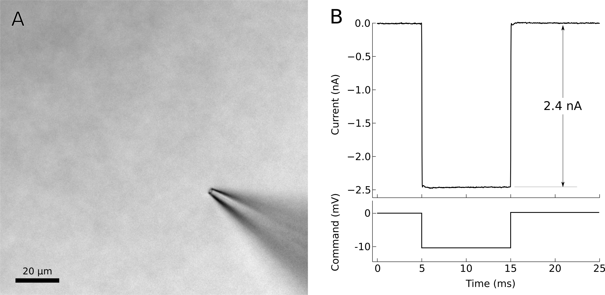
Figure 7. Voltage-clamp recording from cell-attached pipette before (dashed line) and after (solid line) adjusting the pipette capacitance compensation. The seal resistance has increased to 1.6 GΩ. A) Photo of patch pipette in bath. B) Voltage clamp command and current recording from patch pipette in bath. The voltage clamp requires 2.4 nA of current to effect a 10 mV pulse, indicating a pipette resistance of 4.2 MΩ.
Into tissue
With the pipette tip still above the surface of the slice, switch to a high-power objective. If the pipette tip is no longer visible, you may need to move the tip a small distance until it appears in the view. Be cautious–if you cannot see the pipette, it is easy to accidentally drive it into the slice or the objective. Once the tip is visible, proceed slowly down toward the surface of the slice, continuously refocusing to keep the tip in view.
For most situations, it is acceptable to simply center the pipette tip over the position of the target cell and descend directly downward to the cell. For tougher, myelinated tissue or for deeper cells, it may be advantageous to push the pipette in diagonally along its axis. This will avoid some amount of tissue compression that may result from going straight downward. Most micromanipulators can be configured for this purpose.
As the pipette tip enters the surface of the slice, you should immediately see the tissue gently spread away due to the pressure in the pipette. If you do not see this, then it is likely the tip is already clogged or there is insufficient pressure (and this pipette should be immediately discarded). Too much spread however is not a good sign, as it means that you are flooding the slice with the electrode solution. Depending on the solution, this can depolarize nearby cells, and the mechanical action of the flow may also disrupt the tissue. If this occurs, reduce the pressure.
As you proceed closer to the cell, you may encounter obstacles such as fibers or other cells. The positive pressure will push some obstacles out of your way, while other obstacles will need to be avoided. Some trial and error may be necessary at first. Remember, the goal is to arrive at the target cell with a clean pipette tip. Positive pressure makes this possible, but some situations will require finesse as well.
Near cell
When the pipette tip is within 10 μm or so of the target cell, correct the amplifier’s pipette offset again. Press the tip slowly into the center of the cell to form a visible dimple (figures 8A, 9). This dimple is your indication that there is indeed nothing else between the pipette and your cell. Release the pressure on the pipette and wait while monitoring the resistance of the electrode. The cell membrane should immediately come into contact with the electrode tip and begin to form a seal.
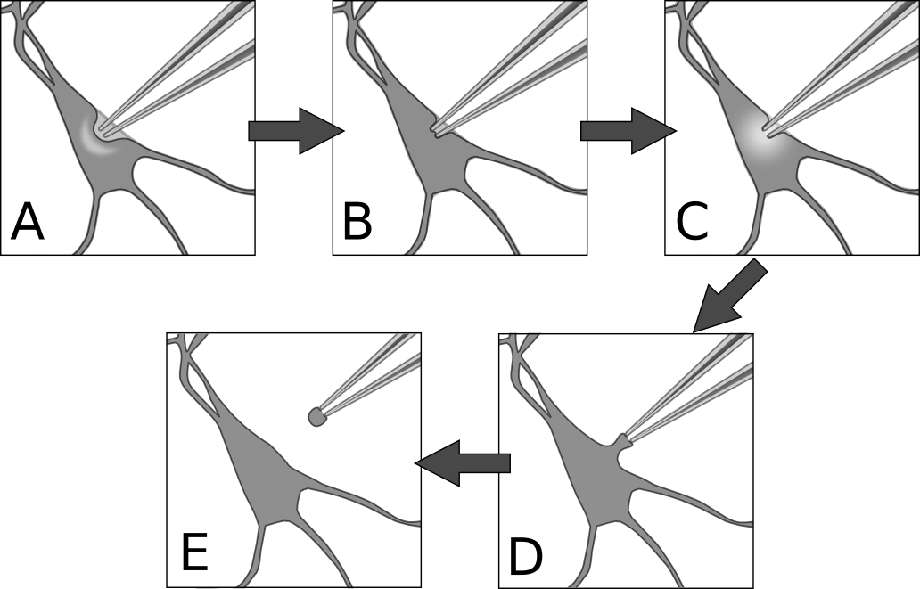
Figure 8. Patch procedure. A) Approach the cell with positive pressure in the pipette. The surface of the cell should form a visible dimple. B) Release pressure on pipette, then apply gentle suction to seal the membrane against the pipette. This is the cell-attached configuration. C) Apply sharp suction to the pipette to rupture the membrane, granting electrical access to the cell interior. This is the whole-cell configuration. D) From whole-cell, pull the pipette very gently away from the cell until E) the membrane separates and re-closes. This is the outside-out configuration.
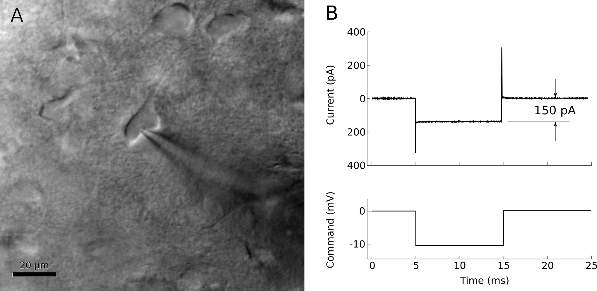
Figure 9. Left: A ‘dimpled’ cell immediately before being patched. Right: voltage-clamp recording shortly after releasing pipette pressure. The resistance at the pipette tip has increased to 66MΩ.
The membrane that has adhered to the pipette tip may spontaneously rupture, so it is important to prepare for this. After the seal resistance has increased past about 100 MΩ, voltage-clamp the pipette near the estimated resting potential of the cell, less the junction potential (for example, if a typical cell rests at -75mV and the junction potential is -12 mV, voltage clamp the pipette at -63 mV with brief steps to -73 mV). The resistance should continue to increase over a few seconds to a minute, going from a few MΩ to over 1 GΩ (figure 10). If resistance is not increasing quickly enough, gentle suction on the pipette can encourage a seal to form. If your software allows, it can be very helpful to watch the pipette resistance plotted over time.
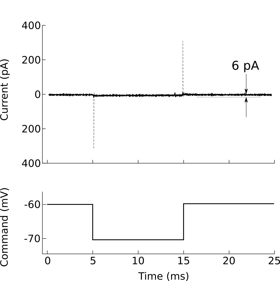
Figure 10. Voltage-clamp recording from cell-attached pipette before (dashed line) and after (solid line) adjusting the pipette capacitance compensation. The seal resistance has increased to 1.6 GΩ.
After forming a gigaohm seal, the pipette is considered “cell attached” (figure 8B). In this mode, it is possible to cleanly record action potentials from the patched cell, but little else should be visible. If your amplifier has built-in pipette capacitance compensation, now is the perfect time to adjust those settings (your amplifier manual should discuss this in detail). This will minimize the transients at the beginning and end of the voltage command step (figure 10).
Break-in
Once a gigaohm seal has been formed, access to the cell can be obtained. Apply brief pulses of suction to break the membrane within the lumen of the pipette (figure 8C). There are several ways to do this. In our lab, we typically use a 1 cc tuberculin syringe to create the suction, using small, quick, pulls on the plunger (0.01-0.03 cc displacements). The negative pressure needed to break into the cell varies with cell type, the preparation, and the pipette tip diameter and taper. Under the best conditions, a displacement of less than 0.1 cc is sufficient to provide a clean break in. Once the break in is achieved, the negative pressure is immediately released. A traditional way to apply suction is to use a mouth-pipette tube. This also gives good control of the pressure. Another way is to use a controlled negative pressure generating system, such as a column of water, along with a valve. However, the complexity of such a system may not be worth the effort to maintain it compared to using the simpler methods. Many amplifiers also offer “zap” and current pulse controls that can be used to try to break the luminal membrane by voltage-breakdown. However, we have not found these to be very effective in the cochlear nucleus or auditory cortex, and when access to the cell is achieved it has high resistance and is not stable.
When whole-cell access is obtained, the membrane current trace will consist of a fast transient current that decays back towards the baseline (figure 11). The amplitude of this transient is inversely proportional to the series resistance (lower resistances generate larger transients), while the time constant of the transient decay is approximately the product of the series resistance and the effective cell capacitance seen by the electrode. The access resistance should be low. Using -10 mV steps, a -1 nA peak current would correspond to 10 MΩ access and 2 nA to 5 MΩ (as follows from Ohm’s law). The time constant corresponds to the speed of the uncompensated voltage clamp and the fast component, corresponding to charging of the soma, usually should be well under 1 ms.
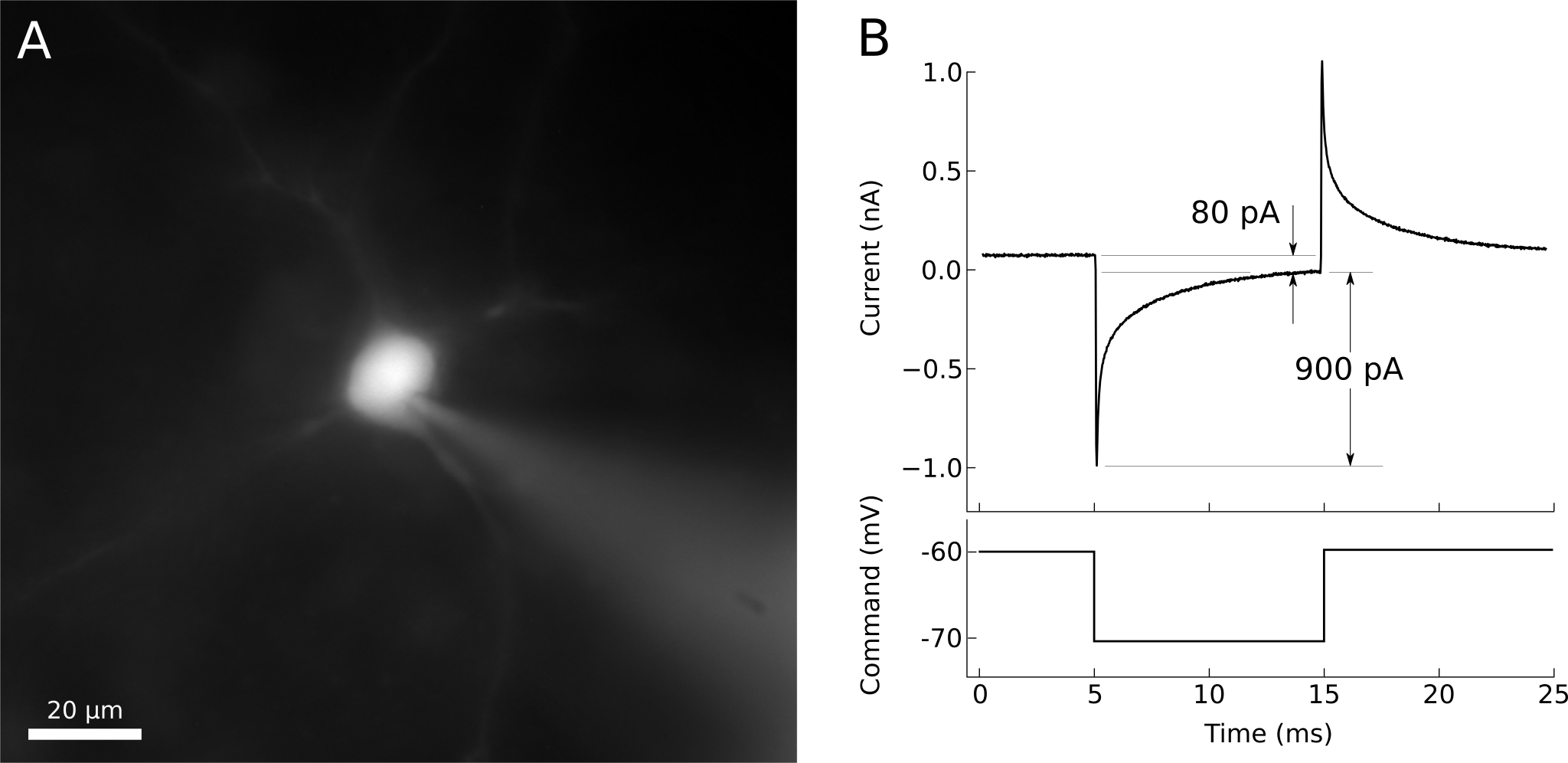
Figure 11. A) Whole-cell patched neuron filled with fluorescent dye. B) Voltage-clamp recording from the same neuron. The steady-state current is about 80 pA, indicating an input resistance of 125 MΩ. The peak of the charging transient is 900 pA past the steady-state, indicating an access resistance of 11 MΩ.
Compensating series resistance and whole cell capacitance
In an ideal voltage clamp, the membrane potential at the patched cell is exactly equal to the requested command voltage. In practice, several factors prevent perfect control of the membrane potential. The small tip of the electrode, combined with cell debris inside the tip, creates a series resistance between the interior of the electrode and the interior of the cell. When current is passed through this series resistance, it results in a voltage difference, so that the resulting membrane potential is no longer equal to the command voltage, but is shifted in a direction that depends on the sign of the current flowing through the electrode at any instant in time. When currents are large, the resistance of the bath electrode may also contribute to this error. Series resistance, when combined with the capacitance of the pipette and of the cell, also introduces a complex low-pass filter that affects how rapidly the voltage at the cell can be changed, and how rapidly the amplifier can detect changes in the cell voltage.
Voltage clamp amplifiers include compensation circuitry that attempts to correct these effects by including a feedback circuit that takes into account the series resistance and cell capacitance, and injects current through the electrode in an attempt to faithfully follow the command voltage. This compensation is essential for experiments that require precise control of the membrane potential and accurate recordings of fast or large currents. It also effectively increases the bandwidth of the clamp, resulting in tighter control of membrane potential during rapid changes in membrane conductance.
The drawbacks to series resistance compensation are that it introduces additional high-frequency noise to the recording, and it is prone to producing oscillations that may damage or destroy the cell if configured incorrectly. For recordings that require very low noise, where the currents are slow, and where a voltage error can be tolerated or is demonstrably small (e.g., measuring small currents where the voltage error is also small), it may be preferable to disable series resistance compensation.
The accuracy of compensation is limited by the extent to which the user is able to adjust the settings to closely reflect the electrical circuit of the pipette and cell. The details for configuring series resistance compensation are found in the manuals of the amplifiers, and because the compensation circuitry varies between amplifiers, those recommendations should be followed. A few important points are in order however. First, any cell with an extended dendritic tree will have a capacitive transient that has multiple time constants. However, the amplifiers are all designed to compensate a single time constant, e.g., a spherical cell body with no processes. Thus, care in adjustment must be used to focus on the correct (somatic) time constant. Second, stable recording conditions need to be attained. Any change in access resistance, or even the bath fluid level, can affect the conditions needed for optimal compensation, and will result at best in incorrect compensation, and at the worst in the system going into oscillation and destroying the cell.
At this point, we wish to raise an important limitation of voltage clamp that is all too often ignored in the literature. Only the point of the cell immediately adjacent to the electrode is properly “voltage-clamped”. There is a large and local spatial gradient over which clamp fidelity decreases, usually on the order of 100 μm or so (see Fig. 12). This can be partially corrected by using the amplifier’s compensation circuitry and by using electrode solution that blocks ion channels to increase the electrotonic space constant of the cell. This issue has been discussed by a number of authors over the years (Spruston et al., 1993; Williams and Mitchell, 2008). In most central neurons, even under the best conditions, only the cell body and proximal ~50 μm of the dendrite is under good control of the voltage clamp. Thus, it may be advisable to record in current clamp to minimize the potential for voltage clamp problems, or if appropriate, patch recordings directly from dendrites might be considered.
Even though the entire neuron cannot be clamped, recording in a voltage clamp mode has several advantages for examining synaptic responses. The clamp keeps the membrane potential relatively constant and below spike threshold, so that synaptic inputs are not likely to drive spikes unexpectedly. In addition, voltage clamp can largely remove the effect of membrane capacitance from conductance changes generated near the recording electrode, which can improve the signal-to-noise ratio for detection and measurements of synaptic inputs, especially when measuring single quantal events such as miniature excitatory or inhibitory postsynaptic potentials. Finally, even though dendritic synaptic events are not fully clamped, relative changes can be measured under different conditions in individual cells, while holding the membrane potential (and synaptic driving force) constant. However, this requires careful consideration of the potential influence of any manipulations on the quality of the clamp and on non-uniform changes in driving force across the dendritic tree.
Inside-out, outside-out
Outside out patches (figure 8D, E) are very useful in evaluating the voltage-dependence of ion channels, and the kinetics of neurotransmitter receptors. These patches have a very low capacitance, and can be well controlled under voltage clamp. They can be pulled from cells in slices, including from fine dendrites. A major advantage of using isolated membrane patches is that the space clamp problem is eliminated. A second advantage is that the site where the channels with particular currents are located can be determined. Disadvantages include the fact that the channel function may be disturbed by wash-out of essential proteins or intracellular ions, or even by introducing an unusual curvature to the patch membrane.
To pull an outside-out patch, first obtain a whole-cell recording (figure 8C). We find that the best patches are pulled within about 10 minutes of accessing the whole-cell configuration, and this provides time to perhaps fill the cell with a dye and to obtain a characterization of the intrinsic physiology. Next, switch the amplifier to voltage-clamp, holding the cell at -60 mV, and provide 10-50 msec long voltage pulses going to -70 mV. It is best to not compensate the amplifier at this point, as visualization of the access resistance and clamp time constant is better obtained by watching the uncompensated currents on an oscilloscope. Begin forming the patch by slowly drawing the pipette away from the cell, at a rate of a few μm per 10 seconds, stopping frequently, in a direction normal to the cell surface at the point of contact (figure 8D). Watching the oscilloscope, you should see an increase in access resistance, as indicated by a decrease in the peak current at the beginning and end of the step, once the pipette is more than about 5 μm from the cell, and a thin bridge of membrane may be visible connecting the pipette to the cell. Continue pulling slowly until the capacitive charging transient at the beginning and end of the voltage pulse becomes very small, and the input resistance of the patch increases as indicated by a decrease in the small steady-state current during the step. The holding current should be less than a few 10’s of pA. You should be able to continue pulling the pipette away and up so that the tip is in the bath above the slice (figure 8E). At this point you have an outside out patch. Applying voltage steps may reveal small currents (10-200 pA), especially with depolarization. Loss of the patch is indicated by a large increase in the holding current and noisy traces.
Note that this procedure can also result in a resealing of the membrane of the cell that the patch was pulled from, and it is often possible to image the cell after recordings from the patch are complete.
Running the experiment
When the cell is patched, you are ready to run your experiment. Patched cells can be temperamental, so it is important to monitor the health of the cell for the duration of the experiment. The major indicators of a failing cell are decreased or increased resting membrane potential (10-15 mV above or below the typical resting potential) and decreased input resistance. These can be monitored by periodically recording the response to current or voltage pulses similar to the procedure used during patching. Alternatively, the cell can be continuously monitored by generating an audible signal from the amplifier.
Additionally, access resistance may increase during the experiment. Although some increase in access is normal, it may cause problems if it continues to increase past 15-20 MΩ in current clamp, or by more than 8-10% in voltage-clamp. Applying very brief, gentle pulses of pressure to the patch pipette may help lower the access resistance, but can also rupture the patch seal.
In some experiments, it is desirable to voltage clamp cells at a membrane potential that is well away from the normal resting potential. For example, to measure currents through NMDA receptors, it is common to clamp the cells at a positive potential, such as +40 mV. Even with Cs-based electrodes, we find that many types of cells to not tolerate being held at positive potentials for more than about 10 seconds at a time. It is usually best to step the cell between a normal holding potential and the positive potential, and apply stimuli during the positive step. Subtraction of traces with and without stimulation may be needed when using such a protocol, as Cs+ does not completely block all potassium currents, and some time-dependent current may remain.
Data analysis
Patch-clamp experiments most commonly generate time-series analog signal recordings (for example, a 1-dimensional array of membrane voltage or current values). These signals are analyzed using a variety of general signal processing techniques as well as less common techniques devised specifically for analysis of neuronal signals. Given a model of the system we are studying (be it a channel, membrane, neuron, or circuit), the objective of any analysis is to measure one or more parameters of the model from signals in the recording. However, the presence of noise and other interfering signals can make this challenging.
Prior to analysis for signals of interest, it is common to digitally filter the recording to remove unwanted noise and offsets. To remove a baseline offset, it is usually sufficient to subtract the mean or median value derived from a quiescent period of the recording. Bessel or Butterworth filters are frequently used to remove both high-frequency noise and low-frequency baseline fluctuations. Any filtering must be applied with caution to avoid altering those aspects of the signal that are to be measured. For example, many filters introduce frequency-dependent phase delays that can affect the measurements of event timing in the signal. Filtering can also generate ringing artifacts in response to rapid changes in the incoming signal or noise spikes. They can also alter the apparent kinetics of rapidly activating currents measured under voltage clamp, such as occurs with voltage-gated sodium and calcium conductances, and some fast synaptic conductances. In general, it is wise to always check that the chosen filtering (or any automated analysis, for that matter) produces the expected results for a set of known inputs, by always checking filtered signals and the subsequent analysis results manually.
Signals of interest in patch clamp recordings can be divided roughly into two categories: evoked events, and spontaneous events. Evoked events are somewhat easier to analyze because their timing usually follows a predictable delay with respect to the stimulus (electric shock, photostimulation, etc.). Evoked events include excitatory and inhibitory postsynaptic currents, action potentials, and direct perturbations of the membrane potential or holding current. Such events are analyzed to characterize their shape in some way. For example, sudden shifts in membrane potential may be fit to exponential decay curves to determine their time constant; action potentials are measured for their amplitude, width, afterhyperpolarization depth, rising and falling slopes, and other criteria; and postsynaptic conductances are analyzed for amplitude, latency, rising and falling kinetics, or total charge transfer.
Analysis of spontaneous (or otherwise poorly timed) events requires extra effort because the timing of events must be determined before they can be measured. In some cases, it may be difficult to unambiguously distinguish events from background noise, or to separate overlapping events. Numerous techniques for event detection have been developed. Most of these work by filtering the signal such that each event is reduced to a single, sharp spike that can be clearly distinguished from the background noise. The timing of these spikes is then detected by searching for regions of the signal that exceed a predefined threshold. A commonly used and more sophisticated analysis uses a template matching algorithm (Clements and Bekkers, 1997). In this approach, a short template with the expected event shape is slid across the trace in time, and the error in the fit (with the baseline and peak amplitude as the adjustable parameters) is returned at each point in time. The regions with the best fits that exceed a statistical criterion are then identified for subsequent analysis. An alternate treatment that can be used in current clamp recordings uses deconvolution to estimate the time course of a current from the voltage traces (Richardson and Silberberg, 2008). This method can be useful for isolating and measuring the amplitudes of overlapping events.